4.2 High degree polynomial interpolation#
Suppose we approximate \(f(x)\) using its polynomial interpolant \(p_{n}(x)\) obtained from \((n+1\)) data points. We then increase the number of data points, and update \(p_{n}(x)\) accordingly. The central question we want to discuss is the following: as the number of nodes (data points) increases, does \(p_{n}(x)\) become a better approximation to \(f(x)\) on \([a,b]?\) We will investigate this question numerically, using a famous example: Runge’s function, given by \(f(x)=\frac{1}{1+x^2}\).
We will interpolate Runge’s function using polynomials of various degrees, and plot the function, together with its interpolating polynomial and the data points. We are interested to see what happens as the number of data points, and hence the degree of the interpolating polynomial, increases.
import numpy as np
import matplotlib.pyplot as plt
%matplotlib inline
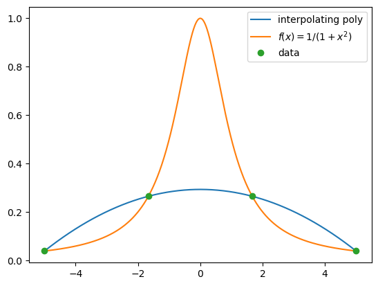
We start with taking four equally spaced \(x\)-coordinates between -5 and 5, and plot the corresponding interpolating polynomial and Runge’s function. Matplotlib allows typing mathematics in captions of a plot using Latex. (Latex is a typesetting program this book is written with.) Latex commands need to be enclosed by a pair of dollar signs, in addition to a pair of quotation marks.
def newton(x, y, z):
    m = x.size # here m is the number of data points, not the degree
    # of the polynomial
    a = diff(x, y)
    sum = a[0]
    pr = 1.0
    for j in range(m-1):
        pr *= (z-x[j])
        sum += a[j+1]*pr
    return sum
def diff(x, y):
    m = x.size # here m is the number of data points.
    # the degree of the polynomial is m-1
    a = np.zeros(m)
    for i in range(m):
        a[i] = y[i]
    for j in range(1, m):
        for i in np.flip(np.arange(j,m)):
            a[i] = (a[i]-a[i-1]) / (x[i]-x[i-(j)])
    return a
f = lambda x: 1/(1+x**2)
xi = np.linspace(-5, 5, 4) # x-coordinates of the data, 4 points equally spaced from
#-5 to 5 in increments of 10/3
yi = f(xi) # the corresponding y-coordinates
xaxis = np.linspace(-5, 5, 1000)
runge = f(xaxis) # Runge's function values
interp = newton(xi, yi, xaxis)
plt.plot(xaxis, interp, label='interpolating poly')
plt.plot(xaxis, runge, label="$f(x)=1/(1+x^2)$")
plt.plot(xi, yi, 'o', label='data')
plt.legend(loc='upper right');

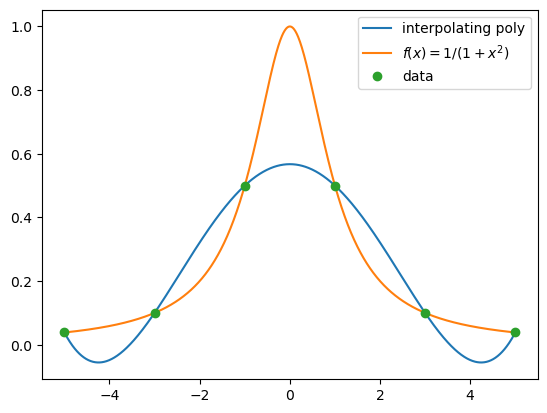
Next, we increase the number of data points to 6.
xi = np.linspace(-5, 5, 6) # 6 equally spaced values from -5 to 5
yi = f(xi) # the corresponding y-coordinates
interp = newton(xi, yi, xaxis)
plt.plot(xaxis, interp, label='interpolating poly')
plt.plot(xaxis, runge, label="$f(x)=1/(1+x^2)$")
plt.plot(xi, yi, 'o', label='data')
plt.legend(loc='upper right');

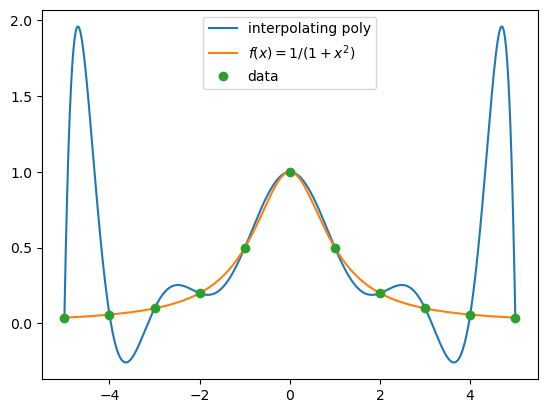
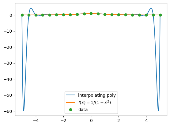
The next two graphs plot interpolating polynomials on 11 and 21 equally spaced data.
xi = np.linspace(-5, 5, 11) # 11 equally spaced values from -5 to 5
yi = f(xi) # the corresponding y-coordinates
interp = newton(xi, yi, xaxis)
plt.plot(xaxis, interp, label='interpolating poly')
plt.plot(xaxis, runge, label="$f(x)=1/(1+x^2)$")
plt.plot(xi, yi, 'o', label='data')
plt.legend(loc='upper center');

xi = np.linspace(-5, 5, 21) # 21 equally spaced values from -5 to 5
yi = f(xi) # the corresponding y-coordinates
interp = newton(xi, yi, xaxis)
plt.plot(xaxis, interp, label='interpolating poly')
plt.plot(xaxis, runge, label="$f(x)=1/(1+x^2)$")
plt.plot(xi, yi, 'o', label='data')
plt.legend(loc='lower center');

We observe that as the degree of the interpolating polynomial increases, the polynomial has large oscillations toward the end points of the interval. In fact, it can be shown that for any \(x\) such that \(3.64<|x|<5, \sup_{n\geq 0} |f(x)-p_n(x)|=\infty\), where \(f\) is Runge’s function.
This troublesome behavior of high degree interpolating polynomials improves significantly, if we consider data with \(x\)-coordinates that are not equally spaced. Consider the interpolation error of Theorem 22:
Perhaps surprisingly, the right-hand side of the above equation is not minimized when the nodes, \(x_i\), are equally spaced! The set of nodes that minimizes the interpolation error is the roots of the so-called Chebyshev polynomials. The placing of these nodes is such that there are more nodes towards the end points of the interval, than the middle. We will learn about Chebyshev polynomials in Chapter 6 Approximation Theory. Using Chebyshev nodes in polynomial interpolation avoids the diverging behavior of polynomial interpolants as the degree increases, as observed in the case of Runge’s function, for sufficiently smooth functions.
Below is a comparison of the interpolations using equally spaced and Chebyshev nodes as the number of data points increases. No deterioration of interpolation quality is observed in the case of Chebyshev nodes.
Show code cell source
from IPython.display import display
from matplotlib.animation import FuncAnimation
from IPython.display import HTML

# Newton Divided Difference Interpolation Method
def NewtonDivDiffInterp(x, y):
    """
    Computes coefficients of interpolating polynomial
    x: the x coordinate of the data points
    y: the y coordinate of the data points
    return: the coefficients $c$ of
    """
    if x.size != y.size:
        print('x and y should have the same size!')
        stop

    n = x.size
    v = np.zeros((n,n))
    # Fill in y column
    for j in range(n):
        v[j,0] = y[j]

    # Fill in all the other columns i:
    for i in range(1, n):
        for j in range(0, n-i):
            v[j,i] = (v[j+1,i-1]-v[j,i-1])/(x[j+i]-x[j])

    c = np.zeros(n,)
    for i in range(n):
        c[i] = v[0, i]

    return c

def nest(d,c,x,b):
    """
    Evaluates polynomial from nested form using Horner's Method
    base points need to be passed in.
    Input:
    d: degree of polynomial
    c: array of d+1 coefficients (constant term first)
    x: x-coordinate at which to evaluate
    """

    y = c[d]
    for i in range(d-1,-1,-1):
        y = y*(x-b[i])+c[i]

    return y

xf = np.linspace(-1, 1, 100)
# use a dropdown or some other widgets to choose a range of functions
yf = 1/(1+12*xf**2)

fig, (ax1, ax2) = plt.subplots(1, 2, figsize=(12,6))
ax1.set_xlim(-1, 1)
ax2.set_xlim(-1, 1)
def animate(i):
    ax1.clear()
    ax2.clear()
    x = np.cos(((2*np.arange(1,i+1)-1)*np.pi)/(2*(i)))
    y = 1./(1+12*x**2)
    c = NewtonDivDiffInterp(x, y)
    xp = np.linspace(-1, 1, 100)
    yp = nest(i-1, c, xp, x)
    ax1.plot(xf, yf, c='b')
    ax1.plot(xp, yp, c='r')
    ax1.plot(x, y, 'o')
    ax1.set_title('Interpolation with '+ str(i) +' Chebyshev points')
    ax1.legend(['f(x)', 'Interpolating poly', 'Data'])


    x = np.linspace(-1, 1, i)
    # change the following line for another function
    y = 1./(1+12*x**2)
    c = NewtonDivDiffInterp(x, y)
    xp = np.linspace(-1, 1, 100)
    yp = nest(i-1, c, xp, x)
    ax2.plot(xf, yf, c='b')
    ax2.plot(xp, yp, c='r')
    ax2.plot(x, y, 'o')
    ax2.set_title('Interpolation with '+ str(i) +' uniform points')
    ax2.legend(['f(x)', 'Interpolating poly', 'Data'])

plt.close()
anim = FuncAnimation(fig, animate, frames=range(2,31), interval=1500)
HTML(anim.to_jshtml())
Divided differences and derivatives#
The following theorem shows the similarity between divided differences and derivatives.
Theorem 24
Suppose \(f\in C^{n}[a,b]\) and \(x_{0},x_{1},...,x_{n}\) are distinct numbers in \([a,b].\) Then there exists \(\xi\in(a,b)\) such that
To prove this theorem, we need the generalized Rolle’s theorem.
Theorem 25 (Rolle’s theorem)
Suppose \(f\) is a differentiable function on \((a,b).\) If \(f(a)=f(b),\) then there exists \(c\in(a,b)\) such that \(f'(c)=0\).
Theorem 26 (Generalized Rolle’s theorem)
Suppose \(f\) has \(n\) derivatives on \((a,b).\) If \(f(x)=0\) at \((n+1)\) distinct numbers \(x_{0},x_{1},...,x_{n}\in[a,b]\), then there exists \(c\in(a,b)\) such that \(f^{(n)}(c)=0\).
Proof of Theorem 24.
Consider the function \(g(x)=p_{n}(x)-f(x).\) Observe that \(g(x_{i})=0\) for \(i=0,1,...,n.\) From generalized Rolle’s theorem, there exists \(\xi\in(a,b)\) such that \(g^{(n)}(\xi)=0,\) which implies
Since \(p_{n}(x)=f[x_{0}]+f[x_{0},x_{1}](x-x_{0})+\cdots+f[x_{0},...,x_{n}](x-x_{0})\cdots(x-x_{n-1})\), \(p_{n}^{(n)}(x)\) equals \(n!\) times the leading coefficient \(f[x_{0},...,x_{n}].\) Therefore
