5.4 Multiple integrals

The numerical quadrature methods we have discussed can be generalized to higher dimensional integrals. We will consider the two-dimensional integral

\[\begin{equation*} \int\int_{R}f(x,y)dA. \end{equation*}\]

The domain \(R\) determines the difficulty in generalizing the one-dimensional formulas we learned before. The simplest case would be a rectangular domain \(R=\{(x,y)|a\leq x\leq b,c\leq y\leq d\}\). We can then write the double integral as the iterated integral

\[\begin{equation*} \int\int_{R}f(x,y)dA=\int_{a}^{b}\left(\int_{c}^{d}f(x,y)dy\right)dx. \end{equation*}\]

Consider a numerical quadrature rule

\[\begin{equation*} \int_{a}^{b}f(x)dx\approx\sum_{i=1}^{n}w_{i}f(x_{i}). \end{equation*}\]

Apply the rule using \(n_{2}\) nodes to the inner integral to get the approximation

\[\begin{equation*} \int_{a}^{b}\left(\sum_{j=1}^{n_{2}}w_{j}f(x,y_{j})\right)dx \end{equation*}\]

where the \(y_{j}\)’s are the nodes. Rewrite, by interchanging the integral and summation, to get

\[\begin{equation*} \sum_{j=1}^{n_{2}}w_{j}\left(\int_{a}^{b}f(x,y_{j})dx\right) \end{equation*}\]

and apply the quadrature rule again, using \(n_{1}\) nodes, to get the approximation

\[\begin{equation*} \sum_{j=1}^{n_{2}}w_{j}\left(\sum_{i=1}^{n_{1}}w_{i}f(x_{i},y_{j})\right). \end{equation*}\]

This gives the two-dimensional rule

\[\begin{equation*} \int_{a}^{b}\left(\int_{c}^{d}f(x,y)dy\right)dx\approx\sum_{j=1}^{n_{2}}\sum_{i=1}^{n_{1}}w_{i}w_{j}f(x_{i},y_{j}). \end{equation*}\]

For simplicity, we ignored the error term in the above derivation; however, its inclusion is straightforward.

For an example, let’s derive the two-dimensional Gauss-Legendre rule for the integral

(31)\[\int_{0}^{1}\int_{0}^{1}f(x,y)dydx\]

using two nodes for each axis. Note that each integral has to be transformed to \((-1,1).\) Start with the inner integral \(\int_{0}^{1}f(x,y)dy\) and use

\[\begin{equation*} t=2y-1, dt=2dy \end{equation*}\]

to transform it to

\[\begin{equation*} \frac{1}{2}\int_{-1}^{1}f\left(x,\frac{t+1}{2}\right)dt \end{equation*}\]

and apply Gauss-Legendre rule with two nodes to get the approximation

\[\begin{equation*} \frac{1}{2}\left(f\left(x,\frac{-1/\sqrt{3}+1}{2}\right)+f\left(x,\frac{1/\sqrt{3}+1}{2}\right)\right). \end{equation*}\]

Substitute this approximation in (31) for the inner integral to get

\[\begin{equation*} \int_{0}^{1} \frac{1}{2}\left(f\left(x,\frac{-1/\sqrt{3}+1}{2}\right)+f\left(x,\frac{1/\sqrt{3}+1}{2}\right)\right) dx. \end{equation*}\]

Now transform this integral to the domain \((-1,1)\) using

\[\begin{equation*} s=2x-1, ds=2dx \end{equation*}\]

to get

\[\begin{equation*} \frac{1}{4} \int_{-1}^{1}\left(f\left(\frac{s+1}{2},\frac{-1/\sqrt{3}+1}{2}\right)+f\left(\frac{s+1}{2},\frac{1/\sqrt{3}+1}{2}\right)\right) ds. \end{equation*}\]

Apply the Gauss-Legendre rule again to get

(32)\[\begin{split}\begin{align} \frac{1}{4} \Biggl[ & f\left(\frac{-1/\sqrt{3}+1}{2},\frac{-1/\sqrt{3}+1}{2}\right)+f\left(\frac{-1/\sqrt{3}+1}{2},\frac{1/\sqrt{3}+1}{2}\right) \nonumber \\ &+f\left(\frac{1/\sqrt{3}+1}{2},\frac{-1/\sqrt{3}+1}{2}\right)+f\left(\frac{1/\sqrt{3}+1}{2},\frac{1/\sqrt{3}+1}{2}\right) \Biggr]. \end{align}\end{split}\]

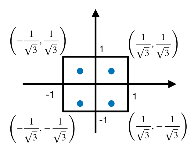
Figure 12 displays the nodes used in this calculation.

Fig. 12 Nodes of double Gauss-Legendre rule.

Next we derive the two-dimensional Simpson’s rule for the same integral, \(\int_{0}^{1}\int_{0}^{1}f(x,y)dydx,\) using \(n=2\), which corresponds to three nodes in the Simpson’s rule (recall that \(n\) is the number of nodes in Gauss-Legendre rule, but \(n+1\) is the number of nodes in Newton-Cotes formulas).

The inner integral is approximated as

\[\begin{equation*} \int_0^1 f(x,y)dy \approx \frac{1}{6} \left( f(x,0)+4f(x,0.5)+f(x,1) \right). \end{equation*}\]

Substitute this approximation for the inner integral in \(\int_{0}^{1}\left(\int_{0}^{1}f(x,y)dy\right)dx\) to get

\[\begin{equation*} \frac{1}{6} \int_0^1 \left( f(x,0)+4f(x,0.5)+f(x,1) \right) dx. \end{equation*}\]

Apply Simpson’s rule again to this integral with \(n=2\) to obtain the final approximation:

(33)\[\begin{split}\begin{align} \frac{1}{6} \Biggl[ \frac{1}{6} &\biggl( f(0,0)+4f(0,0.5)+f(0,1)+4(f(0.5,0)+4f(0.5,0.5)+f(0.5,1)) \nonumber \\ &+f(1,0)+4f(1,0.5)+f(1,1) \biggr) \Biggr]. \end{align}\end{split}\]

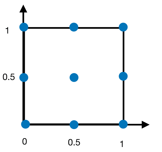
Figure 13 displays the nodes used in the above calculation.

Fig. 13 Nodes of double Simpson’s rule

For a specific example, consider the integral

\[\begin{equation*} \int_0^1 \int_0^1 \left(\frac{\pi}{2} \sin \pi x \right)\left(\frac{\pi}{2} \sin \pi y \right) dy dx. \end{equation*}\]

This integral can be evaluated exactly, and its value is 1. It is used as a test integral for numerical quadrature rules. Evaluating Equations (32) and (33) with \(f(x,y)= \left(\frac{\pi}{2} \sin \pi x \right)\left(\frac{\pi}{2} \sin \pi y \right)\), we obtain the approximations given in the table below:

Simpson’s rule (9 nodes)	Gauss-Legendre (4 nodes)	Exact integral
\(1.0966\)	\(0.93685\)	\(1\)

The Gauss-Legendre rule gives a slightly better estimate than Simpson’s rule, but using less than half the number of nodes.

The approach we have discussed can be extended to regions that are not rectangular, and to higher dimensions. More details, including algorithms for double and triple integrals using Simpson’s and Gauss-Legendre rule, can be found in Burden et al. [2016].

There is however, an obvious disadvantage of the way we have generalized one-dimensional quadrature rules to higher dimensions. Imagine a numerical integration problem where the dimension is 360; such high dimensions appear in some problems from financial engineering. Even if we used two nodes for each dimension, the total number of nodes would be \(2^{360}\), which is about \(10^{100},\) a number too large. In very large dimensions, the only general method for numerical integration is the Monte Carlo method.

Monte Carlo Method

The Monte Carlo method approximates the integral \(\int_0^1 f(x)dx\) using the function average \(\frac{1}{n} \sum_{i=1}^n f(x_i)\), where \(x_i\) are random numbers (from the uniform distribution) between 0 and 1. Most mathematical software have built-in functions that generate random numbers 1. The generalization to higher dimensional integrals is straightforward:

(34)\[\begin{align} \int_{(0,1)^s} f(x)dx\approx \frac{1}{n} \sum_{i=1}^{n}f(x_i), \end{align}\]

where the components of the \(s\)-dimensional vector \(x_i=(x_{i,1},x_{i,2},\ldots,x_{i,s})\) are pseudorandom numbers between 0 and 1.

Consider the two-dimensional integral we discussed before

\[\begin{align*} \int_{a}^{b}\int_{c}^{d}f(x,y)dydx. \end{align*}\]

To use Monte Carlo to estimate this integral, we first have to transform the integration domain to \((0,1)^2\). Using the substitution

\[\begin{align*} u=\frac{x-a}{b-a}, du=\frac{dx}{b-a} \text{ and } v=\frac{y-c}{d-c}, dv=\frac{dy}{d-c}, \end{align*}\]

we obtain

\[\begin{align*} \int_{a}^{b}\int_{c}^{d}f(x,y)dydx = (b-a)(d-c) \int_{0}^{1}\int_{0}^{1}f(a+(b-a)u,c+(d-c)v)dvdu. \end{align*}\]

We can now apply the Monte Carlo method to the integral with domain \((0,1)^2\) to obtain the estimate

(35)\[\begin{align} \int_{a}^{b}\int_{c}^{d}f(x,y)dydx\approx\frac{(b-a)(d-c)}{n}\sum_{i=1}^{n}f(a+(b-a)u_{i},c+(d-c)v_{i}) \end{align}\]

where \(u_{i},v_{i}\) are pseudorandom numbers from \((0,1).\) In Python, the function numpy.random.rand() generates a pseudorandom number from the uniform distribution between 0 and 1. The following code takes the endpoints of the intervals \(a,b,c,d,\) and the number of nodes \(n\) (which is called the sample size in the Monte Carlo literature) as inputs, and returns the estimate for the integral using (35)).

import numpy as np

def mc(f, a, b, c, d, n):
    sum = 0.
    for i in range(n):
        sum += f(a+(b-a)*np.random.rand(),
                 c+(d-c)*np.random.rand())*(b-a)*(d-c)
    return sum/n

Let’s use Monte Carlo to estimate the integral \(\int_0^1 \int_0^1 \left(\frac{\pi}{2} \sin \pi x \right)\left(\frac{\pi}{2} \sin \pi y \right) dy dx\). Using a sample size of \(n=500\) we get:

mc(lambda x,y: (np.pi**2/4)*np.sin(np.pi*x)*np.sin(np.pi*y),
   0, 1, 0, 1, 500)

1.0322218582619718

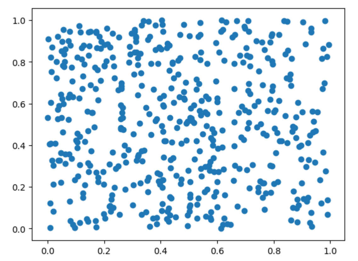
The convergence of the function averages to the integral in (34) is a consequence of the strong law of large numbers of probability theory. From the central limit theorem, it follows that the rate of convergence is \(O(1/\sqrt{n})\), which is independent of the dimension \(s\). The only condition \(f\) has to satisfy for the convergence to hold is that the integral of \(f^2\) is finite. Figure 14 displays 500 pseudorandom vectors from the unit square: these are the vectors at which Monte Carlo computes the function averages.

Fig. 14 Monte Carlo: 500 pseudorandom vectors

Example 49

Capstick and Keister [1996] discuss some high dimensional test integrals, some with analytical solutions, motivated by physical applications such as the calculation of quantum mechanical matrix elements in atomic, nuclear, and particle physics. One of the integrals with a known solution is

\[\begin{equation*} \int_{\mathbb{R}^s} \cos (||\boldsymbol{t}||)) e^{-||\boldsymbol{t}||^2} dt_1 dt_2 \dotsb dt_s \end{equation*}\]

where \(||\boldsymbol{t}||=(t_1^2+\dotsc +t_s^2)^{1/2}\). This integral can be transformed to an integral over the \(s\)-dimensional unit cube as

(36)\[\begin{align} \pi^{s/2} \int_{(0,1)^s} \cos \left[ \left( \frac{(F^{-1}(x_1))^2+\dotsc +(F^{-1}(x_s))^2}{2} \right)^{1/2} \right] dx_1 dx_2 \dotsb dx_s \end{align}\]

where \(F^{-1}\) is the inverse of the cumulative distribution function of the standard normal distribution:

\[\begin{equation*} F(x)=\frac{1}{(2\pi)^{1/2}} \int_{-\infty}^x e^{-w^2/2}dw. \end{equation*}\]

We will estimate the integral (36) by Monte Carlo as

\[\begin{equation*} \frac{\pi^{s/2}}{n} \sum_{i=1}^n \cos \left[ \left( \frac{(F^{-1}(x^{(i)}_1))^2+\dotsc +(F^{-1}(x^{(i)}_s))^2}{2} \right)^{1/2} \right] \end{equation*}\]

where \(\boldsymbol{x}^{(i)}=(x^{(i)}_1, \dotsc, x^{(i)}_s)\) is an \(s\)-dimensional vector of uniform random numbers between 0 and 1.

import numpy as np

import matplotlib.pyplot as plt
%matplotlib inline

The following algorithm, known as the Beasley-Springer-Moro algorithm Glasserman [2013], gives an approximation to \(F^{-1}(x)\).

def invNormal(u):
    # Beasley-Springer-Moro algorithm
    a0 = 2.50662823884
    a1 = -18.61500062529
    a2 = 41.39119773534
    a3 = -25.44106049637
    b0 = -8.47351093090
    b1 = 23.08336743743
    b2 = -21.06224101826
    b3 = 3.13082909833
    c0 = 0.3374754822726147
    c1 = 0.9761690190917186
    c2 = 0.1607979714918209
    c3 = 0.0276438810333863
    c4 = 0.0038405729373609
    c5 = 0.0003951896511919
    c6 = 0.0000321767881768
    c7 = 0.0000002888167364
    c8 = 0.0000003960315187
    
    y = u-0.5
    if np.abs(y)<0.42:
        r = y*y
        x = y*(((a3*r+a2)*r+a1)*r+a0)/((((b3*r+b2)*r+b1)*r+b0)*r+1)
    else:
        r = u
        if y>0:
            r = 1-u
        r = np.log(-np.log(r))
        x = c0+r*(c1+r*(c2+r*(c3+r*(c4+r*(c5+r*(c6+r*(c7+r*c8)))))))
        if y<0:
            x = -x
    return x

The following is the Monte Carlo estimate of the integral. It takes the dimension \(s\) and the sample size \(n\) as inputs.

def mc(s, n):
    est = 0
    for j in range(n):
        sum = 0
        for i in range(s):
            sum += (invNormal(np.random.rand()))**2
        est += np.cos((sum/2)**0.5)
    return np.pi**(s/2)*est/n

The exact value of the integral for \(s=25\) is \(-1.356914\times 10^6\). The following code computes the relative error of the Monte Carlo estimate with sample size \(n\).

relerror = lambda n: np.abs(mc(25,n)+1.356914*10**6)/(1.356914*10**6)

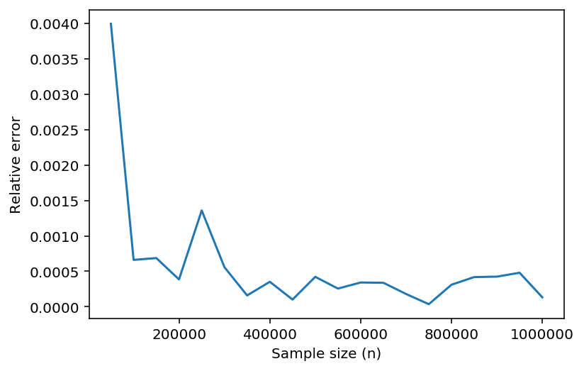
Let’s plot the relative error of some Monte Carlo estimates. First, we generate sample sizes from 50,000 to 1,000,000 in increments of 50,000.

samples = [n for n in range(50000,1000001, 50000)]

For each sample size, we compute the relative error, and then plot the results.

error = [relerror(n) for n in samples]

---------------------------------------------------------------------------
KeyboardInterrupt                         Traceback (most recent call last)
Cell In[10], line 1
----> 1 error = [relerror(n) for n in samples]

Cell In[10], line 1, in <listcomp>(.0)
----> 1 error = [relerror(n) for n in samples]

Cell In[8], line 1, in <lambda>(n)
----> 1 relerror = lambda n: np.abs(mc(25,n)+1.356914*10**6)/(1.356914*10**6)

Cell In[7], line 6, in mc(s, n)
      4     sum = 0
      5     for i in range(s):
----> 6         sum += (invNormal(np.random.rand()))**2
      7     est += np.cos((sum/2)**0.5)
      8 return np.pi**(s/2)*est/n

KeyboardInterrupt: 

plt.plot(samples, error)
plt.xlabel('Sample size (n)')
plt.ylabel('Relative error');

Fig. 15 Monte Carlo relative error for the integral (36).

Exercise 5.4-1

A test integral used in comparing quadrature rules is

\[\begin{equation*} \int_{(0,1)^s} f(x_1,\ldots,x_s)dx_1\ldots dx_s \end{equation*}\]

where

\[\begin{equation*} f(x_1,\ldots,x_s)=\prod_{i=1}^s \frac{|4x_i-2|+1}{2}. \end{equation*}\]

The true value of the integral is one. Use Monte Carlo to estimate the integral when \(s=10\), using sample sizes from 50,000 to 1,000,000, in increments of 50,000, and plot the absolute value of the error against the sample size.

BFB16

R.L. Burden, D. Faires, and A.M. Burden. Numerical Analysis. Cengate, 10th edition, 2016.

CK96

S. Capstick and B.D. Keister. Multidimensional quadrature algorithms at higher degree and/or dimension. Journal of Computational Physics, 123:267–273, 1996.

Gla13

P. Glasserman. Monte Carlo methods in Financial Engineering. Springer, 2013.

---

1

A better word is pseudorandom numbers: numbers that look like a sequence of random numbers, but generated using a computer algorithm.