6.3 Orthogonal polynomials and least squares

Our discussion in this section will mostly center around the continuous least squares problem; however, the discrete problem can be approached similarly. Consider the set \(C^0[a,b]\), the set of all continuous functions defined on \([a,b],\) and \(\mathbf{P_n},\) the set of all polynomials of degree at most \(n\) on \([a,b].\) These two sets are vector spaces, the latter a subspace of the former, under the usual operations of function addition and multiplying by a scalar. An inner product on this space is defined as follows: given \(f,g\in C^0[a,b]\)

(54)\[\begin{equation} \left\langle f,g\right\rangle =\int_{a}^{b}w(x)f(x)g(x)dx \end{equation}\]

and the norm of a vector under this inner product is

\[\begin{equation*} \left\Vert f\right\Vert =\left\langle f,f\right\rangle ^{1/2}=\left(\int_{a}^{b}w(x)f^{2}(x)dx\right)^{1/2}. \end{equation*}\]

Let’s recall the definition of an inner product: it is a real valued function with the following properties:

1. \(\left\langle f,g\right\rangle =\left\langle g,f\right\rangle \)

2. \(\left\langle f,f\right\rangle \geq0,\) with the equality only when \(f\equiv0\)

3. \(\left\langle \beta f,g\right\rangle =\beta\left\langle f,g\right\rangle \) for all real numbers \(\beta\)

4. \(\left\langle f_{1}+f_{2},g\right\rangle =\left\langle f_{1},g\right\rangle +\left\langle f_{2},g\right\rangle \)

The mysterious function \(w(x)\) in (54) is called a weight function. Its job is to assign different importance to different regions of the interval \([a,b]\). The weight function is not arbitrary; it has to satisfy some properties.

Definition 17

A nonnegative function \(w(x)\) on \([a,b]\) is called a weight function if

1. \(\int_{a}^{b}|x|^{n}w(x)dx\) is integrable and finite for all \(n\geq0\)

2. If \(\int_{a}^{b}w(x)g(x)dx=0\) for some \(g(x)\geq0,\) then \(g(x)\) is identically zero on \((a,b).\)

With our new terminology and set-up, we can write the least squares problem as follows:

Problem (Continuous least squares) Given \(f\in C^0[a,b],\) find a polynomial \(P_n(x)\in\mathbf{P_n}\) that minimizes

\[\begin{equation*} \int_{a}^{b}w(x)(f(x)-P_n(x))^{2}dx=\left\langle f(x)-P_n(x),f(x)-P_n(x)\right\rangle. \end{equation*}\]

We will see this inner product can be calculated easily if \(P_n(x)\) is written as a linear combination of orthogonal basis polynomials: \(P_{n}(x)=\sum_{j=0}^{n}a_{j}\phi_{j}(x)\).

We need some definitions and theorems to continue with our quest. Let’s start with a formal definition of orthogonal functions.

Definition 18

Functions \(\{\phi_{0},\phi_{1},...,\phi_{n}\}\) are orthogonal for the interval \([a,b]\) and with respect to the weight function \(w(x)\) if

\[\begin{equation*} \left\langle \phi_{j},\phi_{k}\right\rangle =\int_{a}^{b}w(x)\phi_{j}(x)\phi_{k}(x)dx=\begin{cases} 0 & \text{if }j\neq k\\ \alpha_{j}>0 & \text{if }j=k \end{cases} \end{equation*}\]

where \(\alpha_{j}\) is some constant. If, in addition, \(\alpha_{j}=1\) for all \(j\), then the functions are called orthonormal.

How can we find an orthogonal or orthonormal basis for our vector space? Gram-Schmidt process from linear algebra provides the answer.

Theorem 33 (Gram-Schmidt process)

Given a weight function \(w(x)\), the Gram-Schmidt process constructs a unique set of polynomials \(\phi_{0}(x),\phi_{1}(x),...,\phi_{n}(x)\) where the degree of \(\phi_{i}(x)\) is \(i,\) such that

\[\begin{equation*} \left\langle \phi_{j},\phi_{k}\right\rangle =\begin{cases} 0 & \text{if }j\neq k\\ 1 & \text{if }j=k \end{cases} \end{equation*}\]

and the coefficient of \(x^{n}\) in \(\phi_{n}(x)\) is positive.

Let’s discuss two orthogonal polynomials that can be obtained from the Gram-Schmidt process using different weight functions.

Example 55 (Legendre Polynomials)

If \(w(x)\equiv1\) and \([a,b]=[-1,1]\), the first four polynomials obtained from the Gram-Schmidt process, when the process is applied to the monomials \(1,x,x^2,x^3,...\), are:

\[\begin{equation*} \phi_{0}(x)=\sqrt{\frac{1}{2}},\phi_{1}(x)=\sqrt{\frac{3}{2}}x,\phi_{2}(x)=\frac{1}{2}\sqrt{\frac{5}{2}}(3x^{2}-1), \phi_{3}(x) = \frac{1}{2}\sqrt{\frac{7}{2}}(5x^3-3x). \end{equation*}\]

Often these polynomials are written in its orthogonal form; that is, we drop the requirement \(\left\langle \phi_{j},\phi_{j}\right\rangle =1\) in the Gram-Schmidt process, and we scale the polynomials so that the value of each polynomial at 1 equals 1. The first four polynomials in that form are

\[\begin{equation*} L_{0}(x)=1,L_{1}(x)=x,L_{2}(x)=\frac{3}{2}x^{2}-\frac{1}{2},L_{3}(x)=\frac{5}{2}x^{3}-\frac{3}{2}x. \end{equation*}\]

These are the Legendre polynomials, polynomials we first discussed in Gaussian quadrature, Section 5.3 Gaussian quadrature1. They can be obtained from the following recursion

\[\begin{equation*} L_{n+1}(x)=\frac{2n+1}{n+1}xL_{n}(x)-\frac{n}{n+1}L_{n-1}(x), \end{equation*}\]

\(n=1,2,\ldots\), and they satisfy

\[\begin{equation*} \left\langle L_{n},L_{n}\right\rangle =\frac{2}{2n+1}. \end{equation*}\]

Exercise 6.3-1

Show, by direct integration, that the Legendre polynomials \(L_1(x)\) and \(L_2(x)\) are orthogonal.

Example 56 (Chebyshev polynomials)

If we take \(w(x)=(1-x^{2})^{-1/2}\) and \([a,b]=[-1,1]\), and again drop the orthonormal requirement in Gram-Schmidt, we obtain the following orthogonal polynomials:

\[\begin{equation*} T_{0}(x)=1,T_{1}(x)=x,T_{2}(x)=2x^{2}-1,T_{3}(x)=4x^{3}-3x,... \end{equation*}\]

These polynomials are called Chebyshev polynomials and satisfy a curious identity:

\[\begin{equation*} T_{n}(x)=\cos(n\cos^{-1}x),n\geq0. \end{equation*}\]

Chebyshev polynomials also satisfy the following recursion:

\[\begin{equation*} T_{n+1}(x)=2xT_{n}(x)-T_{n-1}(x) \end{equation*}\]

for \(n=1,2,\ldots\), and

\[\begin{equation*} \left\langle T_{j},T_{k}\right\rangle =\begin{cases} 0 & \text{if }j\neq k\\ \pi & \text{if }j=k=0\\ \pi/2 & \text{if }j=k>0. \end{cases} \end{equation*}\]

If we take the first \(n+1\) Legendre or Chebyshev polynomials, call them \(\phi_{0},...,\phi_{n},\) then these polynomials form a basis for the vector space \(\mathbf{P_n}.\) In other words, they form a linearly independent set of functions, and any polynomial from \(\mathbf{P_n}\) can be written as a unique linear combination of them. These statements follow from the following theorem, which we will leave unproved.

Theorem 34

• If \(\phi_{j}(x)\) is a polynomial of degree \(j\) for \(j=0,1,...,n\), then \(\phi_{0},...,\phi_{n}\) are linearly independent.

• If \(\phi_{0},...,\phi_{n}\) are linearly independent in \(\mathbf{P_n}\), then for any \(q(x)\in\mathbf{P_n},\) there exist unique constants \(c_{0},...,c_{n}\) such that \(q(x)=\sum_{j=0}^{n}c_{j}\phi_{j}(x)\).

Exercise 6.3-2

Prove that if \(\{\phi_0,\phi_1,...,\phi_n\}\) is a set of orthogonal functions, then they must be linearly independent.

We have developed what we need to solve the least squares problem using orthogonal polynomials. Let’s go back to the problem statement:

Given \(f\in C^0[a,b],\) find a polynomial \(P_{n}(x)\in\mathbf{P_{n}}\) that minimizes

\[\begin{equation*} E=\int_{a}^{b}w(x)(f(x)-P_{n}(x))^{2}dx=\left\langle f(x)-P_{n}(x),f(x)-P_{n}(x)\right\rangle \end{equation*}\]

with \(P_{n}(x)\) written as a linear combination of orthogonal basis polynomials: \(P_{n}(x)=\sum_{j=0}^{n}a_{j}\phi_{j}(x)\). In the previous section, we solved this problem using calculus by taking the partial derivatives of \(E\) with respect to \(a_{j}\) and setting them equal to zero. Now we will use linear algebra:

\[\begin{align*} E =\left\langle f-\sum_{j=0}^{n}a_{j}\phi_{j},f-\sum_{j=0}^{n}a_{j}\phi_{j}\right\rangle & =\left\langle f,f\right\rangle -2\sum_{j=0}^{n}a_{j}\left\langle f,\phi_{j}\right\rangle +\sum_{i}\sum_{j}a_{i}a_{j}\left\langle \phi_{i},\phi_{j}\right\rangle \\ & =\left\Vert f\right\Vert ^{2}-2\sum_{j=0}^{n}a_{j}\left\langle f,\phi_{j}\right\rangle +\sum_{j=0}^{n}a_{j}^{2}\left\langle \phi_{j},\phi_{j}\right\rangle \\ & =\left\Vert f\right\Vert ^{2}-2\sum_{j=0}^{n}a_{j}\left\langle f,\phi_{j}\right\rangle +\sum_{j=0}^{n}a_{j}^{2}\alpha_{j}\\ & =\textcolor{blue}{\left\Vert f\right\Vert ^{2}-\sum_{j=0}^{n}\frac{\left\langle f,\phi_{j}\right\rangle ^{2}}{\alpha_{j}}}+\textcolor{red}{\sum_{j=0}^{n}\left[\frac{\left\langle f,\phi_{j}\right\rangle }{\sqrt{\alpha_{j}}}-a_{j}\sqrt{\alpha_{j}}\right]^{2}}. \end{align*}\]

Minimizing this expression with respect to \(a_{j}\) is now obvious: simply choose \(a_{j}=\frac{\left\langle f,\phi_{j}\right\rangle }{\alpha_{j}}\) so that the last summation in the above equation, \(\textcolor{red}{\sum_{j=0}^{n}\left[\frac{\left\langle f,\phi_{j}\right\rangle }{\sqrt{\alpha_{j}}}-a_{j}\sqrt{\alpha_{j}}\right]^{2}}\), vanishes. Then we have solved the least squares problem! The polynomial that minimizes the error \(E\) is

(55)\[\begin{equation} P_{n}(x)=\sum_{j=0}^{n}\frac{\left\langle f,\phi_{j}\right\rangle }{\alpha_{j}}\phi_{j}(x) \end{equation}\]

where \(\alpha_{j}=\left\langle \phi_{j},\phi_{j}\right\rangle\). And the corresponding error is

\[\begin{equation*} E=\textcolor{blue}{\left\Vert f\right\Vert ^{2}-\sum_{j=0}^{n}\frac{\left\langle f,\phi_{j}\right\rangle ^{2}}{\alpha_{j}}}. \end{equation*}\]

If the polynomials \(\phi_{0},...,\phi_{n}\) are orthonormal, then these equations simplify by setting \(\alpha_{j}=1\).

We will appreciate the ease at which \(P_{n}(x)\) can be computed using this approach, via formula (55), as opposed to solving the normal equations of (53) when we discuss some examples. But first let’s see the other advantage of this approach: how \(P_{n+1}(x)\) can be computed from \(P_{n}(x)\). In Equation (55), replace \(n\) by \(n+1\) to get

\[\begin{align*} P_{n+1}(x) =\sum_{j=0}^{n+1}\frac{\left\langle f,\phi_{j}\right\rangle }{\alpha_{j}}\phi_{j}(x)&=\underbrace{\sum_{j=0}^{n}\frac{\left\langle f,\phi_{j}\right\rangle }{\alpha_{j}}\phi_{j}(x)}_{P_n(x)}+\frac{\left\langle f,\phi_{n+1}\right\rangle }{\alpha_{n+1}}\phi_{n+1}(x)\\ & =P_{n}(x)+\frac{\left\langle f,\phi_{n+1}\right\rangle }{\alpha_{n+1}}\phi_{n+1}(x), \end{align*}\]

which is a simple recursion that links \(P_{n+1}\) to \(P_{n}\).

Example 57

Find the least squares polynomial approximation of degree three to \(f(x)=e^{x}\) on \((-1,1)\) using Legendre polynomials.

Solution.

Put \(n=3\) in Equation (55) and let \(\phi_j\) be \(L_j\) to get

\[\begin{align*} P_{3}(x)& =\frac{\left\langle f,L_{0}\right\rangle }{\alpha_{0}}L_{0}(x)+\frac{\left\langle f,L_{1}\right\rangle }{\alpha_{1}}L_{1}(x)+\frac{\left\langle f,L_{2}\right\rangle }{\alpha_{2}}L_{2}(x)+\frac{\left\langle f,L_{3}\right\rangle }{\alpha_{3}}L_{3}(x)\\ &=\frac{\left\langle e^{x},1\right\rangle }{2}+\frac{\left\langle e^{x},x\right\rangle }{2/3}x+\frac{\left\langle e^{x},\frac{3}{2}x^{2}-\frac{1}{2}\right\rangle }{2/5}\left(\frac{3}{2}x^{2}-\frac{1}{2}\right)+\frac{\left\langle e^{x},\frac{5}{2}x^{3}-\frac{3}{2}x\right\rangle }{2/7}\left(\frac{5}{2}x^{3}-\frac{3}{2}x\right), \end{align*}\]

where we used the fact that \(\alpha_j=\langle L_j, L_j \rangle = \frac{2}{2n+1}\) (see Example 55). We will compute the inner products, which are definite integrals on \((-1,1)\), using the five-node Gauss-Legendre quadrature we discussed in the previous chapter. The results rounded to four digits are:

\[\begin{gather*} \left\langle e^{x},1\right\rangle =\int_{-1}^{1}e^{x}dx=2.350\\ \left\langle e^{x},x\right\rangle =\int_{-1}^{1}e^{x}xdx=0.7358\\ \left\langle e^{x},\frac{3}{2}x^{2}-\frac{1}{2}\right\rangle =\int_{-1}^{1}e^{x}\left(\frac{3}{2}x^{2}-\frac{1}{2}\right)dx=0.1431\\ \left\langle e^{x},\frac{5}{2}x^{3}-\frac{3}{2}x\right\rangle =\int_{-1}^{1}e^{x}\left(\frac{5}{2}x^{3}-\frac{3}{2}x\right)dx=0.02013. \end{gather*}\]

Therefore

\[\begin{align*} P_{3}(x) & =\frac{2.35}{2}+\frac{3(0.7358)}{2}x+\frac{5(0.1431)}{2}\left(\frac{3}{2}x^{2}-\frac{1}{2}\right)+\frac{7(0.02013)}{2}\left(\frac{5}{2}x^{3}-\frac{3}{2}x\right)\\ & =0.1761x^{3}+0.5366x^{2}+0.9980x+0.9961. \end{align*}\]

Example 58

Find the least squares polynomial approximation of degree three to \(f(x)=e^{x}\) on \((-1,1)\) using Chebyshev polynomials.

Solution.

As in the previous example solution, we take \(n=3\) in Equation (55)

\[\begin{equation*} P_{3}(x)=\sum_{j=0}^{3}\frac{\left\langle f,\phi_{j}\right\rangle }{\alpha_{j}}\phi_{j}(x), \end{equation*}\]

but now \(\phi_j\) and \(\alpha_j\) will be replaced by \(T_j\), the Chebyshev polynomials, and its corresponding constant; see Example 56. We have

\[\begin{align*} P_{3}(x)= \frac{\left\langle e^{x},T_{0}\right\rangle }{\pi}T_{0}(x)+\frac{\left\langle e^{x},T_{1}\right\rangle }{\pi/2}T_{1}(x)+\frac{\left\langle e^{x},T_{2}\right\rangle }{\pi/2}T_{2}(x)+\frac{\left\langle e^{x},T_{3}\right\rangle }{\pi/2}T_{3}(x). \end{align*}\]

Consider one of the inner products,

\[\begin{equation*} \left\langle e^{x},T_{j}\right\rangle =\int_{-1}^{1}\frac{e^{x}T_{j}(x)}{\sqrt{1-x^{2}}}dx \end{equation*}\]

which is an improper integral due to discontinuity at the end points. However, we can use the substitution \(\theta=\cos^{-1}x\) to rewrite the integral as (see Section 5.5 Improper integrals)

\[\begin{equation*} \left\langle e^{x},T_{j}\right\rangle =\int_{-1}^{1}\frac{e^{x}T_{j}(x)}{\sqrt{1-x^{2}}}dx=\int_{0}^{\pi}e^{\cos\theta}\cos(j\theta)d\theta. \end{equation*}\]

The transformed integrand is smooth, and it is not improper, and hence we can use composite Simpson’s rule to estimate it. The following estimates are obtained by taking \(n=20\) in the composite Simpson’s rule:

\[\begin{align*} \left\langle e^{x},T_{0}\right\rangle =\int_{0}^{\pi}e^{\cos\theta}d\theta & =3.977\\ \left\langle e^{x},T_{1}\right\rangle =\int_{0}^{\pi}e^{\cos\theta}\cos\theta d\theta & =1.775\\ \left\langle e^{x},T_{2}\right\rangle =\int_{0}^{\pi}e^{\cos\theta}\cos2\theta d\theta & =0.4265\\ \left\langle e^{x},T_{3}\right\rangle =\int_{0}^{\pi}e^{\cos\theta}\cos3\theta d\theta & =0.06964 \end{align*}\]

Therefore

\[\begin{align*} P_{3}(x) & =\frac{3.977}{\pi}+\frac{3.55}{\pi}x+\frac{0.853}{\pi}(2x^{2}-1)+\frac{0.1393}{\pi}(4x^{3}-3x)\\ & =0.1774x^{3}+0.5430x^{2}+0.9970x+0.9944. \end{align*}\]

Python code for orthogonal polynomials

Computing Legendre polynomials

Legendre polynomials satisfy the following recursion:

\[\begin{equation*} L_{n+1}(x)=\frac{2n+1}{n+1}xL_n(x)-\frac{n}{n+1} L_{n-1}(x) \end{equation*}\]

for \(n=1,2,\dotsc\), with \(L_0(x)=1\), and \(L_1(x)=x\).

The Python code implements this recursion, with a little modification: the index \(n+1\) is shifted down to \(n\), so the modified recursion is: \(L_{n}(x)=\frac{2n-1}{n}xL_{n-1}(x)-\frac{n-1}{n} L_{n-2}(x)\), for \(n=2,3,\dotsc\).

import numpy as np
import matplotlib.pyplot as plt
%matplotlib inline

def leg(x, n):
    if n == 0:
        return 1
    elif n == 1:
        return x
    else:
        return ((2*n-1)/n)*x*leg(x,n-1)-((n-1)/n)*leg(x,n-2)

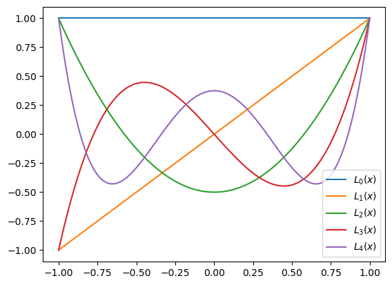
Here is a plot of the first five Legendre polynomials:

xaxis = np.linspace(-1, 1, 200)
legzero = np.array(list(map(lambda x: leg(x,0), xaxis)))
legone = leg(xaxis, 1)
legtwo = leg(xaxis, 2)
legthree = leg(xaxis, 3)
legfour = leg(xaxis, 4)
plt.plot(xaxis, legzero, label='$L_0(x)$')
plt.plot(xaxis, legone, label='$L_1(x)$')
plt.plot(xaxis, legtwo, label='$L_2(x)$')
plt.plot(xaxis, legthree, label='$L_3(x)$')
plt.plot(xaxis, legfour, label='$L_4(x)$')
plt.legend(loc='lower right');

Least-squares using Legendre polynomials

In Example 57, we computed the least squares approximation to \(e^x\) using Legendre polynomials. The inner products were computed using the five-node Gauss-Legendre rule below.

def gauss(f):
    return 0.2369268851*f(-0.9061798459) + 0.2369268851*f(0.9061798459) + \
           0.5688888889*f(0) + 0.4786286705*f(0.5384693101) + \
           0.4786286705*f(-0.5384693101)

The inner product, \(\left\langle e^{x},\frac{3}{2}x^2-\frac{1}{2}\right\rangle =\int_{-1}^{1}e^{x}(\frac{3}{2}x^2-\frac{1}{2})dx\) is computed as

gauss(lambda x: ((3/2)*x**2-1/2)*np.exp(x))

0.1431256282441218

Now that we have a code leg(x,n) that generates the Legendre polynomials, we can do the above computation without explicitly specifying the Legendre polynomial. For example, since \(\frac{3}{2}x^2-\frac{1}{2}=L_2\), we can apply the gauss function directly to \(L_2(x)e^x\):

gauss(lambda x: leg(x,2)*np.exp(x))

0.14312562824412176

The following function polyLegCoeff(f,n) computes the coefficients \(\frac{\left\langle f,L_{j}\right\rangle }{\alpha_{j}}\) of the least squares polynomial \(P_{n}(x)=\sum_{j=0}^{n}\frac{\left\langle f,L_{j}\right\rangle }{\alpha_{j}}L_{j}(x),j=0,1,...,n\), for any \(f\) and \(n\), where \(L_j\) are the Legendre polynomials. The coefficients are the outputs that are returned when the function is finished.

def polyLegCoeff(f, n):
    A = np.zeros(n+1)
    for j in range(n+1):
        A[j] = gauss(lambda x: leg(x,j)*f(x))*(2*j+1)/2
    return A

Once the coefficients are computed, evaluating the polynomial can be done efficiently by using the coefficients. The next function polyLeg(x,n,A) evaluates the least squares polynomial \(P_{n}(x)=\sum_{j=0}^{n}\frac{\left\langle f,L_{j}\right\rangle }{\alpha_{j}}L_{j}(x),j=0,1,...,n\), where the coefficients \(\frac{\left\langle f,L_{j}\right\rangle }{\alpha_{j}}\), stored in \(A\), are obtained from calling the function polyLegCoeff(f,n).

def polyLeg(x, n, A):
    sum = 0.
    for j in range(n+1):
        sum += A[j]*leg(x, j)
    return sum

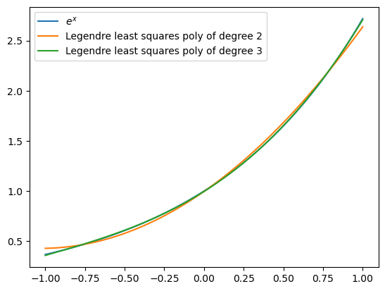
Here we plot \(y=e^x\) together with its least squares polynomial approximations of degree two and three, using Legendre polynomials. Note that every time the function polyLegCoeff is evaluated, a new coefficient array A is obtained.

xaxis = np.linspace(-1, 1, 200)
A = polyLegCoeff(lambda x: np.exp(x), 2)
deg2 = polyLeg(xaxis, 2, A)
A = polyLegCoeff(lambda x: np.exp(x), 3)
deg3 = polyLeg(xaxis, 3, A)
plt.plot(xaxis, np.exp(xaxis), label='$e^x$')
plt.plot(xaxis, deg2, label='Legendre least squares poly of degree 2')
plt.plot(xaxis, deg3, label='Legendre least squares poly of degree 3')
plt.legend(loc='upper left');

Computing Chebyshev polynomials

The following function implements the recursion Chebyshev polynomials satisfy: \(T_{n+1}(x)=2xT_n(x)-T_{n-1}(x)\), for \(n=1,2,...\), with \(T_0(x)=1\) and \(T_1(x)=x\). Note that in the code the index is shifted from \(n+1\) to \(n\).

def cheb(x, n):
    if n == 0:
        return 1
    elif n == 1:
        return x
    else:
        return 2*x*cheb(x,n-1)-cheb(x,n-2)

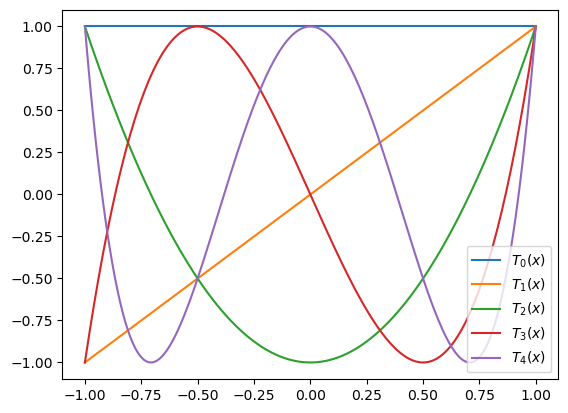
Here is a plot of the first five Chebyshev polynomials:

xaxis = np.linspace(-1, 1, 200)
chebzero = np.array(list(map(lambda x: cheb(x,0), xaxis)))
chebone = cheb(xaxis, 1)
chebtwo = cheb(xaxis, 2)
chebthree = cheb(xaxis, 3)
chebfour = cheb(xaxis, 4)
plt.plot(xaxis, chebzero, label='$T_0(x)$')
plt.plot(xaxis, chebone, label='$T_1(x)$')
plt.plot(xaxis, chebtwo, label='$T_2(x)$')
plt.plot(xaxis, chebthree, label='$T_3(x)$')
plt.plot(xaxis, chebfour, label='$T_4(x)$')
plt.legend(loc='lower right');

Least squares using Chebyshev polynomials

In Example 58, we computed the least squares approximation to \(e^x\) using Chebyshev polynomials. The inner products, after a transformation, were computed using the composite Simpson rule. Below is the Python code for the composite Simpson rule we discussed in the previous chapter.

def compsimpson(f, a, b, n):
    h = (b-a)/n
    nodes = np.zeros(n+1)
    for i in range(n+1):
        nodes[i] = a+i*h
    sum = f(a) + f(b)
    for i in range(2, n-1, 2):
        sum += 2*f(nodes[i])
    for i in range(1, n, 2):
        sum += 4*f(nodes[i])
    return sum*h/3

The integrals in Example 58 were computed using the composite Simpson rule with \(n=20\). For example, the second integral \(\left\langle e^{x},T_{1}\right\rangle =\int_{0}^{\pi}e^{\cos\theta}\cos\theta d\theta\) is computed as:

compsimpson(lambda x: np.exp(np.cos(x))*np.cos(x), 0, np.pi, 20)

1.7754996892121808

Next we write two functions, polyChebCoeff(f,n) and polyCheb(x,n,A). The first function computes the coefficients \(\frac{\left\langle f,T_{j}\right\rangle }{\alpha_{j}}\) of the least squares polynomial \(P_{n}(x)=\sum_{j=0}^{n}\frac{\left\langle f,T_{j}\right\rangle }{\alpha_{j}}T_{j}(x),j=0,1,...,n\), for any \(f\) and \(n\), where \(T_j\) are the Chebyshev polynomials. The coefficients are returned as the output of the first function.

The integral \(\left\langle f,T_{j}\right\rangle\) is transformed to the integral \(\int_0^\pi f(\cos \theta)\cos(j\theta)d\theta\), similar to the derivation in Example 58, and then the transformed integral is computed using the composite Simpson’s rule by polyChebCoeff.

def polyChebCoeff(f, n):
    A = np.zeros(n+1)
    A[0] = compsimpson(lambda x: f(np.cos(x)), 0, np.pi, 20)/np.pi
    for j in range(1, n+1):
        A[j] = compsimpson(lambda x: f(np.cos(x))*np.cos(j*x), 0, np.pi, 20)*2/np.pi
    return A

def polyCheb(x, n, A):
    sum = 0.
    for j in range(n+1):
        sum += A[j]*cheb(x, j)
    return sum

Next we plot \(y=e^x\) together with polynomial approximations of degree two and three using Chebyshev basis polynomials.

xaxis = np.linspace(-1, 1, 200)
A = polyChebCoeff(lambda x: np.exp(x), 2)
deg2 = polyCheb(xaxis, 2, A)
A = polyChebCoeff(lambda x: np.exp(x), 3)
deg3 = polyCheb(xaxis, 3, A)
plt.plot(xaxis, np.exp(xaxis), label='$e^x$')
plt.plot(xaxis, deg2, label='Chebyshev least squares poly of degree 2')
plt.plot(xaxis, deg3, label='Chebyshev least squares poly of degree 3')
plt.legend(loc='upper left');

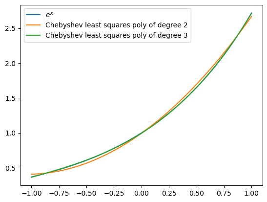
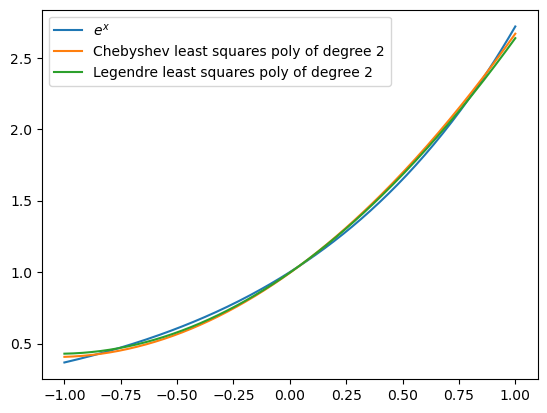
The cubic Legendre and Chebyshev approximations are difficult to distinguish from the function itself. Let’s compare the quadratic approximations obtained by Legendre and Chebyshev polynomials. Below, you can see visually that Chebyshev does a better approximation at the end points of the interval. Is this expected?

xaxis = np.linspace(-1, 1, 200)
A = polyChebCoeff(lambda x: np.exp(x), 2)
cheb2 = polyCheb(xaxis, 2, A)
A = polyLegCoeff(lambda x: np.exp(x), 2)
leg2 = polyLeg(xaxis, 2, A)
plt.plot(xaxis, np.exp(xaxis), label='$e^x$')
plt.plot(xaxis, cheb2, label='Chebyshev least squares poly of degree 2')
plt.plot(xaxis, leg2, label='Legendre least squares poly of degree 2')
plt.legend(loc='upper left');

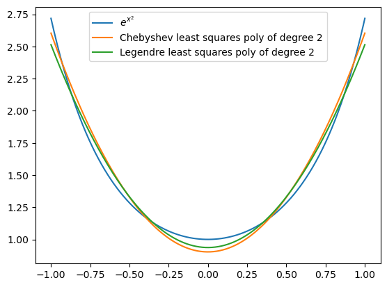
In the following, we compare second degree least squares polynomial approximations for \(f(x)=e^{x^2}\). Compare how good the Legendre and Chebyshev polynomial approximations are in the midinterval and toward the endpoints.

f = lambda x: np.exp(x**2)
xaxis = np.linspace(-1, 1, 200)
A = polyChebCoeff(lambda x: f(x), 2)
cheb2 = polyCheb(xaxis, 2, A)
A = polyLegCoeff(lambda x: f(x), 2)
leg2 = polyLeg(xaxis, 2, A)
plt.plot(xaxis, f(xaxis), label='$e^{x^2}}$')
plt.plot(xaxis, cheb2, label='Chebyshev least squares poly of degree 2')
plt.plot(xaxis, leg2, label='Legendre least squares poly of degree 2')
plt.legend(loc='upper center');

Exercise 6.3-3

Use Python to compute the least squares polynomial approximations \(P_2(x),P_4(x),P_6(x)\) to \(\sin 4x\) using Chebyshev basis polynomials. Plot the polynomials together with \(\sin 4x\).

---

1

The Legendre polynomials in Section 5.3 Gaussian quadrature differ from these by a constant factor. For example, in Section 5.3 Gaussian quadrature the third polynomial was \(L_2(x)=x^2-\frac{1}{3}\), but here it is \(L_2(x)=\frac{3}{2} (x^2-\frac{1}{3})\). Observe that multiplying these polynomials by a constant does not change their roots (what we were interested in Gaussian quadrature), or their orthogonality.